Saturday, December 13, 2008

Cross Tabs and Pivots, Part 1 – Converting Rows to Columns By Jeff Moden, 2008/08/19

Do you get stuck to find the way converting rows to collumns ?? so.. this is the sollutions :

Introduction:


(This article is dedicated to a good friend and fellow T-SQL warrior, Katrina Wright. We've fought and won many battles together.)


I looked for a definition of what a "Cross Tab" actually is and, after a slight modification, couldn't find a better one than what's in SQL Server 2000 Books Online...


"Sometimes it is necessary to rotate results so that [the data in] columns are presented horizontally and [the data in] rows are presented vertically. This is known as creating a PivotTable®, creating a cross-tab report, or rotating data."


In other words, you can use a Cross Tab or Pivot to convert or transpose information from rows to columns either for reporting or to convert some special long skinny tables known as EAV's or NVP's into a more typical form data.


The purpose of this article is to provide an introduction to Cross Tabs and Pivots and how they can be used to "rotate" data...


Before you say anything...


The reason I'm writing a series of articles on the simple concept of Cross Tabs and Pivots is because of the recent number of requests for this type of information on the SQL Server Central forums... there was a while when not a day went by when two or three such requests were posted each day.


Also, yes, I aware that a lot of this type of "formatting" should be done in the GUI, reporting tool, or maybe even a Spreadsheet. I'm also aware that using EAV/NVP tables isn't considered to be a "best practice". But, like I said about the number of recent number of posts, folks get forced into a corner by their bosses and, if they have to do such a thing, I thought they could use a little help.


Notes of Interest:


I wrote all of the example code and data using Temp Tables just to be safe. Sure, I could have used Table Variables, but they don't really allow for people to do partial runs and they don't all people to look and see what's in the Table Variable after each section. Also, some of the data we'll end up using is a wee bit bigger than what I would normally use a table variable for.


Last but not least, I currently only have SQL Server 2000 and 2005 installed. I indicate which rev each section of code will run on in parenthesis. I'm pretty sure that most of this will work on 2008 and that a good portion of the code for Cross Tabs will also work on 7... but I don't have access to either which means I haven't tested it.


Also, for your convenience, all of the code has been attached in the "Resources" section near the end of the article.


Ok... let's get started...


A simple introduction to Cross Tabs:


The Cross Tab Report example from Books Online is very simple and easy to understand. I've shamelessly borrowed from it to explain this first shot at a Cross Tab.


The Test Data


Basically, the table and data looks like this...


--===== Sample data #1 (#SomeTable1)
--===== Create a test table and some data
CREATE TABLE #SomeTable1
(
Year SMALLINT,
Quarter TINYINT,
Amount DECIMAL(2,1)
)
GO
INSERT INTO #SomeTable1
(Year, Quarter, Amount)
SELECT 2006, 1, 1.1 UNION ALL
SELECT 2006, 2, 1.2 UNION ALL
SELECT 2006, 3, 1.3 UNION ALL
SELECT 2006, 4, 1.4 UNION ALL
SELECT 2007, 1, 2.1 UNION ALL
SELECT 2007, 2, 2.2 UNION ALL
SELECT 2007, 3, 2.3 UNION ALL
SELECT 2007, 4, 2.4 UNION ALL
SELECT 2008, 1, 1.5 UNION ALL
SELECT 2008, 3, 2.3 UNION ALL
SELECT 2008, 4, 1.9
GO


Every row in the code above is unique in that each row contains ALL the information for a given quarter of a given year. Unique data is NOT a requirement for doing Cross Tabs... it just happens to be the condition that the data is in. Also, notice that the 2nd quarter for 2008 is missing.


The goal is to make the data look more like what you would find in a spreadsheet... 1 row for each year with the amounts laid out in columns for each quarter with a grand total for the year. Kind of like this...


... and, notice, we've plugged in a "0" for the missing 2nd quarter of 2008.


Year   1st Qtr 2nd Qtr 3rd Qtr 4th Qtr Total 
------ ------- ------- ------- ------- -----
2006 1.1 1.2 1.3 1.4 5.0
2007 2.1 2.2 2.3 2.4 9.0
2008 1.5 0.0 2.3 1.9 5.7


The KEY to Cross Tabs!


Let's start out with the most obvious... we want a Total for each year. This isn't required for Cross Tabs, but it will help demonstrate what the key to making a Cross Tab is.


To make the Total, we need to use the SUM aggregate and a GROUP BY... like this...


--===== Simple sum/total for each year
SELECT Year,
SUM(Amount) AS Total
FROM #SomeTable1
GROUP BY Year
ORDER BY Year


And, that returns the following...


Year   Total                                    
------ ----------------------------------------
2006 5.0
2007 9.0
2008 5.7


Not so difficult and really nothing new there. So, how do we "pivot" the data for the Quarter?


Let's do this by the numbers...


  1. How many quarters are there per year? Correct, 4.

  2. How many columns do we need to show the 4 quarters per year? Correct, 4.

  3. How many times do we need the Quarter column to appear in the SELECT list to make it show up 4 times per year? Correct, 4.

  4. Now, look at the total column... it gives the GRAND total for each year. What would we have to do to get it to give us, say, the total just for the first quarter for each year? Correct... we need a CASE statement inside the SUM.


Number 4 above is the KEY to doing this Cross Tab... It should be a SUM and it MUST have a CASE to identify the quarter even though each quarter only has 1 value. Yes, if each quarter had more than 1 value, this would still work! If any given quarter is missing, a zero will be substituted.


To emphasize, each column for each quarter is just like the Total column, but it has a CASE statement to trap info only for the correct data for each quarter's column. Here's the code...


--===== Each quarter is just like the total except it has a CASE
-- statement to isolate the amount for each quarter.
SELECT Year,
SUM(CASE WHEN Quarter = 1 THEN Amount ELSE 0 END) AS [1st Qtr],
SUM(CASE WHEN Quarter = 2 THEN Amount ELSE 0 END) AS [2nd Qtr],
SUM(CASE WHEN Quarter = 3 THEN Amount ELSE 0 END) AS [3rd Qtr],
SUM(CASE WHEN Quarter = 4 THEN Amount ELSE 0 END) AS [4th Qtr],
SUM(Amount) AS Total
FROM #SomeTable1
GROUP BY Year


... and that gives us the following result in the text mode (modified so it will fit here)...


Year   1st Qtr 2nd Qtr 3rd Qtr 4th Qtr Total
------ ------- ------- ------- ------- -----
2006 1.1 1.2 1.3 1.4 5.0
2007 2.1 2.2 2.3 2.4 9.0
2008 1.5 .0 2.3 1.9 5.7

Also notice... because there is only one value for each quarter, we could have gotten away with using MAX instead of SUM. Go ahead... try it. We'll use a similar method for normalizing an EAV table in the future.


For most applications, that's good enough. If it's supposed to represent the final output, we might want to make it a little prettier. The STR function inherently right justifies, so we can use that to make the output a little prettier. Please, no hate mail here! I'll be one of the first that formatting of this nature is supposed to be done in the GUI!


--===== We can use the STR function to right justify data and make it prettier.
-- Note that this should really be done by the GUI or Reporting Tool and
-- not in T-SQL
SELECT Year,
STR(SUM(CASE WHEN Quarter = 1 THEN Amount ELSE 0 END),5,1) AS [1st Qtr],
STR(SUM(CASE WHEN Quarter = 2 THEN Amount ELSE 0 END),5,1) AS [2nd Qtr],
STR(SUM(CASE WHEN Quarter = 3 THEN Amount ELSE 0 END),5,1) AS [3rd Qtr],
STR(SUM(CASE WHEN Quarter = 4 THEN Amount ELSE 0 END),5,1) AS [4th Qtr],
STR(SUM(Amount),5,1) AS Total
FROM #SomeTable1
GROUP BY Year


The code above gives us the final result we were looking for...


Year   1st Qtr 2nd Qtr 3rd Qtr 4th Qtr Total 
------ ------- ------- ------- ------- -----
2006 1.1 1.2 1.3 1.4 5.0
2007 2.1 2.2 2.3 2.4 9.0
2008 1.5 0.0 2.3 1.9 5.7

Just to emphasize what the very simple KEY to making a Cross Tab is... it's just like making a Total using SUM and Group By, but we've added a CASE statement to isolate the data for each Quarter.


A simple introduction to Pivots:


Microsoft introduced the PIVOT function in SQL Server 2005. It works about the same (has some limitations) as a Cross Tab. Using the same test table we used in the Cross Tab examples above, let's see how to use PIVOT to do the same thing...


--===== Use a Pivot to do the same thing we did with the Cross Tab
SELECT Year, --(4)
[1] AS [1st Qtr], --(3)
[2] AS [2nd Qtr],
[3] AS [3rd Qtr],
[4] AS [4th Qtr],
[1]+[2]+[3]+[4] AS Total --(5)
FROM (SELECT Year, Quarter,Amount FROM #SomeTable1) AS src --(1)
PIVOT (SUM(Amount) FOR Quarter IN ([1],[2],[3],[4])) AS pvt --(2)
ORDER BY Year


Ok... let's break that code down and figure out what each part does... the items below have numbers in the code above so you can more easily see what's going on...


  1. The FROM clause is actually a derived table. It very simply contains the columns that we want to use in the cross tab from the source table we want to use the pivot on. It will sometimes work as a normal FROM clause with just the table listed instead of a derived table, but most of the time it will not and is unpredictable when it does work.

  2. This is the "Pivot" line. It identifies the aggregate to be used, the column to pivot in the FOR clause, and the list of values that we want to pivot in the IN clause... in this case, the quarter number. Also notice that you must treat those as if they were column names. They must either be put in brackets or double quotes (if the quoted identifier setting is ON).

  3. This is the pivoted SELECT list. Notice that you have to bring everything in the IN clause from (2) up to the SELECT list. Aliasing the column names is optional but usually a good thing to do just to make the output obvious.

  4. You must also bring Year up as the row identifier in the pivot. Think of this as your "anchor" for the rows.

  5. Last but not least, if you want a total for each row in the pivot, you can no longer use just an aggregate. Instead, you must add all the columns together.


When you run the code, you get this...


Year   1st Qtr 2nd Qtr 3rd Qtr 4th Qtr Total
------ ------- ------- ------- ------- -----
2006 1.1 1.2 1.3 1.4 5.0
2007 2.1 2.2 2.3 2.4 9.0
2008 1.5 NULL 2.3 1.9 NULL

Notice the NULL's where there are no values or where a NULL has been added into a total. Remember that anything plus a NULL is still a NULL. All of this occurs because the Pivot doesn't do any substitutions like the Case statements we used in the Cross Tab. To fix this little problem, we have to use COALESCE (or ISNULL) on the columns... every bloody column! So, you end up with code that looks like this...


--===== Converting NULLs to zero's in the Pivot using COALESCE
SELECT Year,
COALESCE([1],0) AS [1st Qtr],
COALESCE([2],0) AS [2nd Qtr],
COALESCE([3],0) AS [3rd Qtr],
COALESCE([4],0) AS [4th Qtr],
COALESCE([1],0) + COALESCE([2] ,0) + COALESCE([3],0) + COALESCE([4],0) AS Total
FROM (SELECT Year, Quarter,Amount FROM #SomeTable1) AS src
PIVOT (SUM(Amount) FOR Quarter IN ([1],[2],[3],[4])) AS pvt
ORDER BY Year


That finally gives us the same result as a Cross Tab sans any right hand justification... again, you'd need to add the STR function to the code to do that.


Year   1st Qtr 2nd Qtr 3rd Qtr 4th Qtr Total
------ ------- ------- ------- ------- -----
2006 1.1 1.2 1.3 1.4 5.0
2007 2.1 2.2 2.3 2.4 9.0
2008 1.5 .0 2.3 1.9 5.7

Readability Comparison


Just for grins, here are both the Cross Tab and the Pivot code real close together so that you can do a comparison...


--===== The Cross Tab example 
SELECT Year,
SUM(CASE WHEN Quarter = 1 THEN Amount ELSE 0 END) AS [1st Qtr],
SUM(CASE WHEN Quarter = 2 THEN Amount ELSE 0 END) AS [2nd Qtr],
SUM(CASE WHEN Quarter = 3 THEN Amount ELSE 0 END) AS [3rd Qtr],
SUM(CASE WHEN Quarter = 4 THEN Amount ELSE 0 END) AS [4th Qtr],
SUM(Amount) AS Total
FROM #SomeTable1
GROUP BY Year

--===== The Pivot Example
SELECT Year,
COALESCE([1],0) AS [1st Qtr],
COALESCE([2],0) AS [2nd Qtr],
COALESCE([3],0) AS [3rd Qtr],
COALESCE([4],0) AS [4th Qtr],
COALESCE([1],0) + COALESCE([2] ,0) + COALESCE([3],0) + COALESCE([4],0) AS Total
FROM (SELECT Year, Quarter,Amount FROM #SomeTable1) AS src
PIVOT (SUM(Amount) FOR Quarter IN ([1],[2],[3],[4])) AS pvt
ORDER BY Year


I'm sure that you'll have a preference, but I like the Cross Tab code better for two reasons... the Cross Tab code is simpler, in my eyes... all I have to remember how to do are those very simple Case statements, I only have to list the values of the pivot columns once, and I don't have to use COALESCE anywhere. The second reason is how simple it is to do a row total.


There's actually several other reasons and one of them is performance. We'll get to performance later, but first let's talk about...


Multiple Aggregations In a Cross Tab (or, "The Problem with Pivots")


We're going to do this section backwards from what we've been doing... we're going to cover how to Pivot multiple aggregations before we cover the equivalent Cross Tab.


A "multiple aggregation Pivot" is just that... we want to show two different aggregates in the Pivot something like this (notice both the Qty and Amt columns have been aggregated)...


Company Year   Q1Amt Q1Qty Q2Amt Q2Qty Q3Amt Q3Qty Q4Amt Q4Qty TotalAmt TotalQty
------- ------ ----- ----- ----- ----- ----- ----- ----- ----- -------- --------
ABC 2006 1.1 2.2 1.2 2.4 1.3 1.3 1.4 4.2 5.0 10.1
ABC 2007 2.1 2.3 2.2 3.1 2.3 2.1 2.4 1.5 9.0 9.0
ABC 2008 1.5 5.1 0.0 0.0 2.3 3.3 1.9 4.2 5.7 12.6
XYZ 2006 2.1 3.6 2.2 1.8 3.3 2.6 2.4 3.7 10.0 11.7
XYZ 2007 3.1 1.9 1.2 1.2 3.3 4.2 1.4 4.0 9.0 11.3
XYZ 2008 2.5 3.9 3.5 2.1 1.3 3.9 3.9 3.4 11.2 13.3


This type of Pivot is a common request so that both aggregates can be viewed for the same time period at the same time. Otherwise, you'd have two completely separate Pivots and you'd have to visually scan back and forth to make simple comparisons. As you'll see the "Problem with Pivots" is that each Pivot can only aggregate one column. To do something like this using Pivots, you have two use two Pivots.


The Test Data


Before we begin, we need some data to test with...


--===== Sample data #2 (#SomeTable2)
--===== Create a test table and some data
CREATE TABLE #SomeTable2
(
Company VARCHAR(3),
Year SMALLINT,
Quarter TINYINT,
Amount DECIMAL(2,1),
Quantity DECIMAL(2,1)
)
GO
INSERT INTO #SomeTable2
(Company,Year, Quarter, Amount, Quantity)
SELECT 'ABC', 2006, 1, 1.1, 2.2 UNION ALL
SELECT 'ABC', 2006, 2, 1.2, 2.4 UNION ALL
SELECT 'ABC', 2006, 3, 1.3, 1.3 UNION ALL
SELECT 'ABC', 2006, 4, 1.4, 4.2 UNION ALL
SELECT 'ABC', 2007, 1, 2.1, 2.3 UNION ALL
SELECT 'ABC', 2007, 2, 2.2, 3.1 UNION ALL
SELECT 'ABC', 2007, 3, 2.3, 2.1 UNION ALL
SELECT 'ABC', 2007, 4, 2.4, 1.5 UNION ALL
SELECT 'ABC', 2008, 1, 1.5, 5.1 UNION ALL
SELECT 'ABC', 2008, 3, 2.3, 3.3 UNION ALL
SELECT 'ABC', 2008, 4, 1.9, 4.2 UNION ALL
SELECT 'XYZ', 2006, 1, 2.1, 3.6 UNION ALL
SELECT 'XYZ', 2006, 2, 2.2, 1.8 UNION ALL
SELECT 'XYZ', 2006, 3, 3.3, 2.6 UNION ALL
SELECT 'XYZ', 2006, 4, 2.4, 3.7 UNION ALL
SELECT 'XYZ', 2007, 1, 3.1, 1.9 UNION ALL
SELECT 'XYZ', 2007, 2, 1.2, 1.2 UNION ALL
SELECT 'XYZ', 2007, 3, 3.3, 4.2 UNION ALL
SELECT 'XYZ', 2007, 4, 1.4, 4.0 UNION ALL
SELECT 'XYZ', 2008, 1, 2.5, 3.9 UNION ALL
SELECT 'XYZ', 2008, 2, 3.5, 2.1 UNION ALL
SELECT 'XYZ', 2008, 3, 1.3, 3.9 UNION ALL
SELECT 'XYZ', 2008, 4, 3.9, 3.4
GO


The Multi-Aggregate Pivot


Like I said... we'll do the Pivot first this time... then we'll show you how easy it is to do using a Cross Tab.


In order to do a single Pivot, you have to have a derived table and a Pivot clause. The "Problem with Pivots" is that you can only Pivot one aggregate per Pivot clause. If you want to Pivot two aggregates as shown at the beginning of this section, you have to make two Pivots and join them as well as adding the necessary columns to the Select list. You already know how to use a single Pivot... Here's how we would do a double Pivot using the data above...


--===== The "Problem with Pivots" is you need to do one Pivot for each aggregate.
-- This code Pivots the Amt and Qty values by quarter.
SELECT amt.Company,
amt.Year,
COALESCE(amt.[1],0) AS Q1Amt,
COALESCE(qty.[1],0) AS Q1Qty,
COALESCE(amt.[2],0) AS Q2Amt,
COALESCE(qty.[2],0) AS Q2Qty,
COALESCE(amt.[3],0) AS Q3Amt,
COALESCE(qty.[3],0) AS Q3Qty,
COALESCE(amt.[4],0) AS Q4Amt,
COALESCE(qty.[4],0) AS Q4Qty,
COALESCE(amt.[1],0)+COALESCE(amt.[2],0)+COALESCE(amt.[3],0)+COALESCE(amt.[4],0) AS TotalAmt,
COALESCE(qty.[1],0)+COALESCE(qty.[2],0)+COALESCE(qty.[3],0)+COALESCE(qty.[4],0) AS TotalQty
FROM (SELECT Company, Year, Quarter, Amount FROM #SomeTable2) t1
PIVOT (SUM(Amount) FOR Quarter IN ([1], [2], [3], [4])) AS amt
INNER JOIN
(SELECT Company, Year, Quarter, Quantity FROM #SomeTable2) t2
PIVOT (SUM(Quantity) FOR Quarter IN ([1], [2], [3], [4])) AS qty
ON qty.Company = amt.Company
AND qty.Year = amt.Year
ORDER BY amt.Company, amt.Year


I don't know about you, but my personal feeling is that's starting to look a bit complicated and it's starting to be more difficult to read. Certainly, if we tried to convert this to dynamic SQL, you'd have your work cut out for you.


Notice that the FROM clause has two nearly identical derived tables and the only difference in the Pivot clauses are the columns being SUMmed. And, take a look at the row totals in the Select list... thank goodness this example only has 4 columns each for Quantity and Amount.


The Multi-Aggregate Cross Tab


We saw how complicated Multi-Aggregate Pivots can get. And the example above was just for two 4 column aggregates... just image what it might look like for three 12 column aggregates!


Let's see how complicated it might be in a Cross Tab...ready?


--===== Doing multiple aggregations in Cross Tabs is as simple as CPR
-- (CPR = Cut, Paste, Replace). AND, the table is "dipped" only
-- once instead of twice so there are NO JOINS to worry about!
SELECT Company,
Year,
SUM(CASE WHEN Quarter = 1 THEN Amount ELSE 0 END) AS Q1Amt,
SUM(CASE WHEN Quarter = 1 THEN Quantity ELSE 0 END) AS Q1Qty,
SUM(CASE WHEN Quarter = 2 THEN Amount ELSE 0 END) AS Q2Amt,
SUM(CASE WHEN Quarter = 2 THEN Quantity ELSE 0 END) AS Q2Qty,
SUM(CASE WHEN Quarter = 3 THEN Amount ELSE 0 END) AS Q3Amt,
SUM(CASE WHEN Quarter = 3 THEN Quantity ELSE 0 END) AS Q3Qty,
SUM(CASE WHEN Quarter = 4 THEN Amount ELSE 0 END) AS Q4Amt,
SUM(CASE WHEN Quarter = 4 THEN Quantity ELSE 0 END) AS Q4Qty,
SUM(Amount) AS TotalAmt,
SUM(Quantity) AS TotalQty
FROM #SomeTable2
GROUP BY Company, Year
ORDER BY Company, Year


How easy is that!? There're no derived tables... no fancy Pivot clauses... no huge lines of code to make simple row totals... and no joins!. It's a breeze to make using a little CPR (Copy, Paste, Replace).


Go back and compare the incredible simplicity of this Cross Tab with the relatively complex Pivot code to do the same thing. I don't know about you, but I won't be using Pivot to do such a simple thing.


"Pre-Aggregation"


I found something very handy in the past... I call it "Pre-Aggregation" and it can be used on either a Cross Tab or a Pivot.


The general purpose of pre-aggregation is to make it very easy to summarize the data and then format the data for display. Sometimes you'll have some complex aggregations that are a bit difficult or impossible to do when mixed with the rotation in the Select list, so the best thing to do is to do the aggregations as a derived table and then rotate the results. For example, if you want to aggregate dates by month, you'll find it's much easier to pre-aggregate the data using a formula to convert all dates to the first of the month. We'll cover more on that subject in the next article on Cross Tabs.


Pre-aggregation is nothing more than doing the aggregation as part of a derived table and then doing a Cross Tab or Pivot on that result. That's all it is.


You'll find pre-aggregation code for both Cross Tabs and Pivots in the next section of code where you'll also find another really good reason for doing pre-aggregation even if you don't need it to solve complexity...


Performance


Ah yes... what about performance? Just because the code looks simple or complex doesn't necessarily mean faster or slower nor fewer or more resources. Here's the full test code I used... I intentionally did NOT calculate Quarters from the date in the Cross Tabs or the Pivots because I wanted to show you just how much of a performance difference a simple tweak here and there can make... the biggest tweaks I made was the use of pre-aggregation and the use of CTE's...


--===== Create and populate a 1,000,000 row test table.
-- Column "RowNum" has a range of 1 to 1,000,000 unique numbers
-- Column "Company" has a range of "AAA" to "BBB" non-unique 3 character strings
-- Column "Amount has a range of 0.0000 to 9999.9900 non-unique numbers
-- Column "Quantity" has a range of 1 to 50,000 non-unique numbers
-- Column "Date" has a range of >=01/01/2000 and <01/01/2010 non-unique date/times
-- Columns Year and Quarter are the similarly named components of Date
-- Jeff Moden


SELECT TOP 1000000 --<<Look! Change this number for testing different size tables
RowNum = IDENTITY(INT,1,1),
Company = CHAR(ABS(CHECKSUM(NEWID()))%2+65)
+ CHAR(ABS(CHECKSUM(NEWID()))%2+65)
+ CHAR(ABS(CHECKSUM(NEWID()))%2+65),
Amount = CAST(ABS(CHECKSUM(NEWID()))%1000000/100.0 AS MONEY),
Quantity = ABS(CHECKSUM(NEWID()))%50000+1,
Date = CAST(RAND(CHECKSUM(NEWID()))*3653.0+36524.0 AS DATETIME),
Year = CAST(NULL AS SMALLINT),
Quarter = CAST(NULL AS TINYINT)
INTO #SomeTable3
FROM Master.sys.SysColumns t1
CROSS JOIN
Master.sys.SysColumns t2

--===== Fill in the Year and Quarter columns from the Date column
UPDATE #SomeTable3
SET Year = DATEPART(yy,Date),
Quarter = DATEPART(qq,Date)

--===== A table is not properly formed unless a Primary Key has been assigned
-- Takes about 1 second to execute.
ALTER TABLE #SomeTable3
ADD PRIMARY KEY CLUSTERED (RowNum)
CREATE NONCLUSTERED INDEX IX_#SomeTable3_Cover1
ON dbo.#SomeTable3 (Company, Year)
INCLUDE (Amount, Quantity, Quarter)
GO
SET STATISTICS TIME OFF
SET STATISTICS IO OFF
GO
---------------------------------------------------------------------------------------------------
--===== "Normal" Cross Tab
PRINT REPLICATE('=',100)
PRINT '=============== "Normal" Cross Tab ==============='
SET STATISTICS IO ON
SET STATISTICS TIME ON
SELECT Company,
Year,
SUM(CASE WHEN Quarter = 1 THEN Amount ELSE 0 END) AS Q1Amt,
SUM(CASE WHEN Quarter = 1 THEN Quantity ELSE 0 END) AS Q1Qty,
SUM(CASE WHEN Quarter = 2 THEN Amount ELSE 0 END) AS Q2Amt,
SUM(CASE WHEN Quarter = 2 THEN Quantity ELSE 0 END) AS Q2Qty,
SUM(CASE WHEN Quarter = 3 THEN Amount ELSE 0 END) AS Q3Amt,
SUM(CASE WHEN Quarter = 3 THEN Quantity ELSE 0 END) AS Q3Qty,
SUM(CASE WHEN Quarter = 4 THEN Amount ELSE 0 END) AS Q4Amt,
SUM(CASE WHEN Quarter = 4 THEN Quantity ELSE 0 END) AS Q4Qty,
SUM(Amount) AS TotalAmt,
SUM(Quantity) AS TotalQty
FROM #SomeTable3
GROUP BY Company, Year
ORDER BY Company, Year
SET STATISTICS TIME OFF
SET STATISTICS IO OFF
---------------------------------------------------------------------------------------------------
--===== "Normal" Pivot
PRINT REPLICATE('=',100)
PRINT '=============== "Normal" Pivot ==============='
SET STATISTICS IO ON
SET STATISTICS TIME ON
SELECT amt.Company,
amt.Year,
COALESCE(amt.[1],0) AS Q1Amt,
COALESCE(qty.[1],0) AS Q1Qty,
COALESCE(amt.[2],0) AS Q2Amt,
COALESCE(qty.[2],0) AS Q2Qty,
COALESCE(amt.[3],0) AS Q3Amt,
COALESCE(qty.[3],0) AS Q3Qty,
COALESCE(amt.[4],0) AS Q4Amt,
COALESCE(qty.[4],0) AS Q5Qty,
COALESCE(amt.[1],0)+COALESCE(amt.[2],0)+COALESCE(amt.[3],0)+COALESCE(amt.[4],0) AS TotalAmt,
COALESCE(qty.[1],0)+COALESCE(qty.[2],0)+COALESCE(qty.[3],0)+COALESCE(qty.[4],0) AS TotalQty
FROM (SELECT Company, Year, Quarter, Amount FROM #SomeTable3) t1
PIVOT (SUM(Amount) FOR Quarter IN ([1], [2], [3], [4])) AS amt
INNER JOIN
(SELECT Company, Year, Quarter, Quantity FROM #SomeTable3) t2
PIVOT (SUM(Quantity) FOR Quarter IN ([1], [2], [3], [4])) AS qty
ON qty.Company = amt.Company
AND qty.Year = amt.Year
ORDER BY amt.Company, amt.Year
SET STATISTICS TIME OFF
SET STATISTICS IO OFF
---------------------------------------------------------------------------------------------------
--===== "Pre-aggregated" Cross Tab
PRINT REPLICATE('=',100)
PRINT '=============== "Pre-aggregated" Cross Tab ==============='
SET STATISTICS IO ON
SET STATISTICS TIME ON
SELECT Company,
Year,
SUM(CASE WHEN Quarter = 1 THEN Amount ELSE 0 END) AS Q1Amt,
SUM(CASE WHEN Quarter = 1 THEN Quantity ELSE 0 END) AS Q1Qty,
SUM(CASE WHEN Quarter = 2 THEN Amount ELSE 0 END) AS Q2Amt,
SUM(CASE WHEN Quarter = 2 THEN Quantity ELSE 0 END) AS Q2Qty,
SUM(CASE WHEN Quarter = 3 THEN Amount ELSE 0 END) AS Q3Amt,
SUM(CASE WHEN Quarter = 3 THEN Quantity ELSE 0 END) AS Q3Qty,
SUM(CASE WHEN Quarter = 4 THEN Amount ELSE 0 END) AS Q4Amt,
SUM(CASE WHEN Quarter = 4 THEN Quantity ELSE 0 END) AS Q4Qty,
SUM(Amount) AS TotalAmt,
SUM(Quantity) AS TotalQty
FROM (SELECT Company,Year,Quarter,SUM(Amount) AS Amount,SUM(Quantity) AS Quantity
FROM #SomeTable3 GROUP BY Company,Year,Quarter) d
GROUP BY Company, Year
ORDER BY Company, Year
SET STATISTICS TIME OFF
SET STATISTICS IO OFF
---------------------------------------------------------------------------------------------------
--===== "Pre-aggregated" Pivot
PRINT REPLICATE('=',100)
PRINT '=============== "Pre-aggregated" Pivot ==============='
SET STATISTICS IO ON
SET STATISTICS TIME ON
SELECT amt.Company,
amt.Year,
COALESCE(amt.[1],0) AS Q1Amt,
COALESCE(qty.[1],0) AS Q1Qty,
COALESCE(amt.[2],0) AS Q2Amt,
COALESCE(qty.[2],0) AS Q2Qty,
COALESCE(amt.[3],0) AS Q3Amt,
COALESCE(qty.[3],0) AS Q3Qty,
COALESCE(amt.[4],0) AS Q4Amt,
COALESCE(qty.[4],0) AS Q5Qty,
COALESCE(amt.[1],0)+COALESCE(amt.[2],0)+COALESCE(amt.[3],0)+COALESCE(amt.[4],0) AS TotalAmt,
COALESCE(qty.[1],0)+COALESCE(qty.[2],0)+COALESCE(qty.[3],0)+COALESCE(qty.[4],0) AS TotalQty
FROM (SELECT Company, Year, Quarter, SUM(Amount) AS Amount FROM #SomeTable3 GROUP BY Company, Year, Quarter) t1
PIVOT (SUM(Amount) FOR Quarter IN ([1], [2], [3], [4])) AS amt
INNER JOIN
(SELECT Company, Year, Quarter, SUM(Quantity) AS Quantity FROM #SomeTable3 GROUP BY Company, Year, Quarter) t2
PIVOT (SUM(Quantity) FOR Quarter IN ([1], [2], [3], [4])) AS qty
ON qty.Company = amt.Company
AND qty.Year = amt.Year
ORDER BY amt.Company, amt.Year
SET STATISTICS TIME OFF
SET STATISTICS IO OFF
---------------------------------------------------------------------------------------------------
--===== "Pre-aggregated" Cross Tab with CTE
PRINT REPLICATE('=',100)
PRINT '=============== "Pre-aggregated" Cross Tab with CTE ==============='
SET STATISTICS IO ON
SET STATISTICS TIME ON
;WITH
ctePreAgg AS
(SELECT Company,Year,Quarter,SUM(Amount) AS Amount,SUM(Quantity) AS Quantity
FROM #SomeTable3
GROUP BY Company,Year,Quarter
)
SELECT Company,
Year,
SUM(CASE WHEN Quarter = 1 THEN Amount ELSE 0 END) AS Q1Amt,
SUM(CASE WHEN Quarter = 1 THEN Quantity ELSE 0 END) AS Q1Qty,
SUM(CASE WHEN Quarter = 2 THEN Amount ELSE 0 END) AS Q2Amt,
SUM(CASE WHEN Quarter = 2 THEN Quantity ELSE 0 END) AS Q2Qty,
SUM(CASE WHEN Quarter = 3 THEN Amount ELSE 0 END) AS Q3Amt,
SUM(CASE WHEN Quarter = 3 THEN Quantity ELSE 0 END) AS Q3Qty,
SUM(CASE WHEN Quarter = 4 THEN Amount ELSE 0 END) AS Q4Amt,
SUM(CASE WHEN Quarter = 4 THEN Quantity ELSE 0 END) AS Q4Qty,
SUM(Amount) AS TotalAmt,
SUM(Quantity) AS TotalQty
FROM ctePreAgg
GROUP BY Company, Year
ORDER BY Company, Year
SET STATISTICS TIME OFF
SET STATISTICS IO OFF
---------------------------------------------------------------------------------------------------
--===== "Pre-aggregated" Pivot with CTE
PRINT REPLICATE('=',100)
PRINT '=============== "Pre-aggregated" Pivot with CTE ==============='
SET STATISTICS IO ON
SET STATISTICS TIME ON
;WITH
ctePreAgg AS
(SELECT Company,Year,Quarter,SUM(Amount) AS Amount,SUM(Quantity) AS Quantity
FROM #SomeTable3
GROUP BY Company,Year,Quarter
)
SELECT amt.Company,
amt.Year,
COALESCE(amt.[1],0) AS Q1Amt,
COALESCE(qty.[1],0) AS Q1Qty,
COALESCE(amt.[2],0) AS Q2Amt,
COALESCE(qty.[2],0) AS Q2Qty,
COALESCE(amt.[3],0) AS Q3Amt,
COALESCE(qty.[3],0) AS Q3Qty,
COALESCE(amt.[4],0) AS Q4Amt,
COALESCE(qty.[4],0) AS Q5Qty,
COALESCE(amt.[1],0)+COALESCE(amt.[2],0)+COALESCE(amt.[3],0)+COALESCE(amt.[4],0) AS TotalAmt,
COALESCE(qty.[1],0)+COALESCE(qty.[2],0)+COALESCE(qty.[3],0)+COALESCE(qty.[4],0) AS TotalQty
FROM (SELECT Company, Year, Quarter, Amount FROM ctePreAgg) AS t1
PIVOT (SUM(Amount) FOR Quarter IN ([1], [2], [3], [4])) AS amt
INNER JOIN
(SELECT Company, Year, Quarter, Quantity FROM ctePreAgg) AS t2
PIVOT (SUM(Quantity) FOR Quarter IN ([1], [2], [3], [4])) AS qty
ON qty.Company = amt.Company
AND qty.Year = amt.Year
ORDER BY amt.Company, amt.Year
SET STATISTICS TIME OFF
SET STATISTICS IO OFF


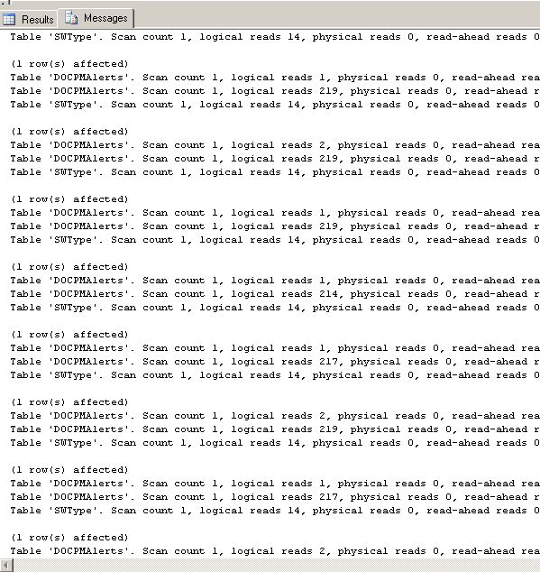
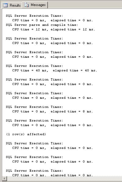
The test code was executed 10 times each for 10k, 100k, and 1 million rows both with and without the index created at the beginning of the code. The averaged results, calculated from a profiler table (not included in the code), are fascinating. The light green cells indicate the fastest run times or the least number of reads. The light blue indicate the second place for the same thing...


Notice that even for "normal" Cross Tabs and Pivots that the only place a Pivot wins in any category is in the paltry 10k row test. The Cross Tab wins everywhere else. That's good news for SQL Server 2000 users because you won't want to change your code if and when you upgrade to SQL Server 2005. Using CTE's helps a bit but not as much as pre-aggregation on the larger row counts does. Again, that's good news for SQL Server 2000 users.


Review


In this article, we learned the basis of how to change rows to columns using both Cross Tabs and Pivot. We've discovered that Cross Tabs are nothing more than simple aggregations that have a built in selection condition in the form of a simple Case statement. We've seen how to use a Pivot to do the same thing as a Cross Tab and, in the process, discovered that they're a bit more complicated to create, read, and understand especially when compared to the simplicity of the Cross Tab code. We've been introduced to the concept of "pre-aggregation and the fact that pre-aggregation can make more complex aggregations both easier to read and to contrive. Through testing, we've found that the Cross Tab beats Pivot code in all but the smallest of tables. Through that same testing, we've also found that pre-aggregation adds a substantial performance gain in all but the smallest of tables.


Last but certainly not least, we've discovered that there's no reason to rewrite properly written Cross Tabs to become Pivots when shifting from SQL Server 2000 to SQL Server 2005. To do so would actually cause a negative impact to performance most of the time.


In the Works...


Coming soon to a forum near you... Dynamic Cross Tabs, EAV/NVP conversions, and more on pre-aggregation.


Thanks for listening folks.


--Jeff Moden


Tuning SQL Server performance via disk arrays and disk partitioning

One of my collections, about MSSQL Server Tunning. Enjoy it...

Author : Denny Cherry, 08.19.2008

As a DBA, much of your focus is on performance tuning SQL Server. But have you spent time to tune the hardware supporting your SQL Server system? Are you using the optimal disk array configuration? Are the disk partitions aligned? This tip discusses how to get your SQL Server hardware performance in top shape – whether the system is already in operation or it's a new setup.


With the massive amount of raw horse power available in today's server class hardware, it's easy to skip over the hardware when it comes to performance tuning the SQL Server database. After all, with so much power available, who cares if something takes a few extra milliseconds to complete? Is anyone really going to notice that extra millisecond?


But what happens when you perform an operation that takes 10 extra milliseconds to complete; and it needs to perform 100 times an hour, for a year? All of a sudden, that 10 milliseconds turns into 2.4 hours. If you perform that operation 1,000 times an hour -- which isn't all that unheard of in a smaller OLTP database -- you are now looking at more than 24 hours of wasted time.


In my particular environment, we run the same stored procedure at least 2,000 times per minute. If that stored procedure takes an extra 10 milliseconds to complete, we are looking at eight hours of lost time daily, or 121 days of lost time per year.


Tune SQL Server by tuning disk arrays


There are a few places to check hardware components when tuning your SQL Server system. The easiest components to check are disk arrays. Typically, disk arrays are where the most time is expended


More on tuning SQL Server performance and hardware:
  • Determining SQL Server database storage requirements

  • Optimize disk configuration in SQL Server

  • Storage area network (SAN) basics every DBA must know


  • waiting for something to happen. There are a couple of ways to tune the disks to improve SQL Server performance. The first is to make sure your disk array has enough spindles to handle the workload that will be placed on it. Second, make sure the disk arrays are in the correct RAID level to offer the best support level for the database.


    While it is true that RAID 10 offers better write performance, in most cases, RAID 10 isn't required for the data files. That said, you should use RAID 10 for your transaction logs and tempdb database, as they are mostly write files. The reason I say not to use RAID 10 for all database files is that RAID 10 is very costly to implement in large disk sizes. This is because for each spindle used for data, a second spindle is used for redundancy.


    Finding out if you need more spindles on an existing system is easy. Open Performance Monitor on the server and add the "Physical Disk" object and the "Current Disk Queue Length" counter. Some queuing is OK; however, there is a tipping point. To find out where the tipping point of "OK queuing" and "too much queuing" is, take the number of disks in the array and multiply it by two. If the result is greater than the maximum value in Performance Monitor, then you have too much queuing. When we talk about the number of disks, we're referring to the number of disks that are actively working with data. If you have a RAID 10 array, this is half the number of disks in the array.


    "Number of Disks" x 2 = Maximum Allowable Queuing


    How to configure the disk array on your new SQL Server system


    When working on a new system without any load on it, making sure you configure your disk array correctly is a little more challenging. If you have another system with the same amount of load on it, you can use that system as a guide. However, if this is the first large system in your environment, then getting it correct can be a bit harder.


    You'll need to look at your database system and the expected transactions per second, and make an educated guess on how many spindles you'll need. When dealing with high-end drives, expect each drive to give you about 100 IOPs to 120 IOPs per second per disk in an OLTP environment. When dealing with SATA drives, expect each drive to give you about 60 IOPs to 80 IOPs per second per disk in an OLTP environment. Those numbers will go up when working in an OLAP environment because OLAP databases put a different kind of load on the disk system. It's a more sequential load, whereas OLTP databases put a random load on the disks.


    Disk partition alignment improves SQL Server performance


    Once you set up your disk array, you'll want to make sure the partition you create is correctly aligned. By default, when Windows (or any other operating system for that matter) creates the partition on a disk or array, the partition is not correctly aligned for peak performance. Disk drives are made up of 1K blocks. The physical disks like to do all their operations in 64-block chunks called clusters. Conveniently, SQL Server likes to do all its operations in 64 K operations -- there are eight 8K blocks in each extent, and SQL does its reads one extent at a time. When the partition is created, the boot sector is created at the beginning of the partition. This boot sector is 32 K in size, causing the 64K operations to be spread between two 64K clusters. This then causes each logical operation to take twice as many physical operations as needed.


    You can see your current alignment offset by using the diskpart application. Open a command prompt and run diskpart.exe. When you are prompted with a DISKPART> prompt, type SELECT DISK n where n is the disk number you want to look at -- the command LIST DISK will give you a list of disks in the machine. After selecting the disk, type in "LIST PARTITION" to get the partition information, including the offset.


    Using disk partition in SQL Server

    Figure 1: Run the DISKPART application to view disk alignment.

    In order to create the partition, you'll need to use the CREATE PARTITION command. The full command is CREATE PARTITION PRIMARY ALIGN=64. This creates the new partition with the 64K offset, aligning the partition into the optimum position for maximum performance.


    Check out part two in this tip series, configuring memory and CPU processing for improved SQL Server performance.

    Tuning SQL Server performance via memory and CPU processing

    After a long journey browsing on internet, finally I found this interesting and usefull article for tunning our MSSQL Database Server. So in this place i re posting to share with you guys.... enjoy it ;)

    Author : Denny Cherry, 09.09.2008
    In my previous tip, Tuning SQL Server performance via disk arrays and disk partitioning, we talked about how important it is to ensure that your storage was set up correctly to optimize SQL Server performance. However, storage isn't the only part of SQL Server hardware that needs special consideration when designing your infrastructure.


    SQL Server memory can also impact performance. While having too much memory in a SQL Server system is a waste of money, having too little memory is extremely detrimental to performance. Unfortunately, determining when you need more memory in the system can be a bit tricky. When memory problems begin, you'll start to see an increase in disk I/O, as well as an increase in disk queuing. You'll also see a decrease in the buffer cache hit ratio and page life expectancy. As memory requirements increase, you may begin to see these error messages in the log file:


  • A significant part of SQL Server process memory has been paged out. This may result in a performance degradation. Duration: %n seconds. Working set (KB): %w, committed (KB): %c, memory utilization: %u.


  • SQL Server has encountered %o occurrence(s) of IO requests taking longer than 15 seconds to complete on file [%f] in database [%d] (%i). The OS file handle is %h. The offset of the latest long IO is: %l.


  • Unfortunately, this is not the only time these errors are reported, so you have to use them along with the performance monitor metrics to determine that memory is actually low.


    When dealing with SQL Server memory issues, there are a few options to resolve the problems. The easiest solution is to increase server memory, which increases the amount of buffer


    More on improving SQL Server performance:
  • Memory configurations for procedure cache and buffer cache
  • Configuring SQL Server memory settings

  • Clustered and non-clustered indexes in SQL Server


  • cache available. This adds to the amount of data in memory and reduces your disk I/O. Other potential solutions include removing clustered indexes for extremely large tables and using only nonclustered indexes for the table, including the Primary Key.


    This will only make a difference when the clustered index is being used for lookups, and clustered index seeks are used. If another index is in use, it will not relieve any memory pressure, as the clustered index won't be in memory. If you're using clustered index scans, then this turns into table scans that load the table into memory instead of the index. If clustered index scans are being performed, then a new nonclustered index may help the situation without removing the index.


    How to monitor CPU queuing


    The CPU is another piece of hardware that can cause potential performance problems. Most people only look at the speed of or number of CPUs. However, just like disks, CPUs can become bottlenecked. If there is a CPU bottleneck, you may not even see the CPU performance at 100%. CPUs have command queues in much the same way that disks have I/O queues. Commands are loaded into a CPU queue and the operation waits for the CPU to become available before performing the operation. As CPUs became faster, we could do things much faster within the CPU, but we could still only do the same number of things at one time. Now, as dual-core, tri-core and quad-core CPUs become available, we can process more commands at one time.


    You can monitor your CPU queue using SQL Server Performance Monitor. You'll find PerfMon under the System object, with the counter name "Processor Queue Length." Pretty much any queue length other than zero indicates a need to increase the number of operations that SQL Server can perform at any one time. It doesn't indicate a need for faster CPUs, but a need for more CPU cores. Today's newest servers support 32 cores per server, and some of the most advanced servers support up to 64 cores -- when chases are scaled together support for 64 cores can be built (available only from certain vendors).


    In parts one and two, I've pointed out a variety of places within the hardware that impact whether your SQL Server system will run at peak performance. These tips are not the be-all, end-all solutions to performance problems. Table design and index tuning always have been and will continue to be extremely important. Today's SQL Server is expected to do more work for more hours of the day, which makes hardware tuning more important to the success of the database platform. With these tools in your arsenal to combat performance problems, you'll be able to get every ounce of performance from the existing hardware with no or minimal hardware upgrades to the platform. But when you do need to make those purchasing decisions, use these tips to make the correct purchasing decisions to get the most upgrade for your dollars spent.


    Tuesday, September 23, 2008

    Export data from SQL Server to Excel

    Problem
    Exporting data from SQL Server to Excel seems like a reasonably simple request. I just need to write out a few reports for users on a regular basis, nothing too fancy, the same basic report with a few different parameters. What native SQL Server options are available to do so? Do I need to learn another tool or can I use some T-SQL commands? Does SQL Server 2005 offer any new options to enhance this process?

    ..Read More

    Solution
    Exporting data from SQL Server to Excel can be achieved in a variety of ways. Some of these options include Data Transformation Services (DTS), SQL Server Integration Services (SSIS) and Bulk Copy (BCP). Data Transformation Services (SQL Server 2000) and SQL Server Integration Services (SQL Server 2005) offers a GUI where widgets can be dragged and dropped Each option has advantages and disadvantages, but all can do the job. It is just a matter of your comfort level with the tools and the best solution to meet the need.

    Another option that is available directly via the T-SQL language is the OPENROWSET command (SQL Server 2000 and SQL Server 2005). This command can be called directly in any stored procedure, script or SQL Server Job from T-SQL. Below outlines the full syntax available:


    Source - SQL Server 2005 Books Online

    Below is a simple example of writing out the Job name and date to Sheet1 of an Excel spreadsheet in either SQL Server 2005 or 2000:


    INSERT INTO OPENROWSET('Microsoft.Jet.OLEDB.4.0',
    'Excel 8.0;Database=C:\testing.xls;',
    'SELECT Name, Date FROM [Sheet1$]')
    SELECT [Name], GETDATE() FROM msdb.dbo.
    sysjobs
    GO

    Using the OPENROWSET command creates two caveats. The first caveat is the need to have an Excel spreadsheet serve as a template in the needed directory with the correct worksheets and columns. Without this the you would receive an error message. The second caveat is that it is necessary to enable the OPENROWSET command with the SQL Server 2005 Surface Area Configuration utility. Note - This step is not needed for SQL Server 2000. With the loop example you could copy and paste the Excel spreadsheet and load the data as needed.

    Although the example above is very simple, you could integrate this simple example into your code. For example, if you had the need to write out a number of reports in the same format, you could loop (WHILE loop or Cursor) over the records and write them out to different Excel spreadsheets based on the name or report type. In addition, you could integrate this code with either SQL Server 2000 mail or Database mail (SQL Server 2005) and mail the results to the users with very little effort and build the process entirely with T-SQL.

    Next Steps

    Getting IO and time statistics for SQL Server queries

    Problem
    If you're like any other DBA or developer in the world, writing sound T-SQL code and performance tuning is one of your primary duties. There are many tools, both native to SQL Server and third-party, that assist you in this endeavor. But in thinking about writing and tuning queries, what should the focus be? For many, the length of time taken to execute the query is "good enough". One focus should be on the resources used by the server, since the length of time taken to execute the query can vary based on other server activity. In addition to using Profiler and Execution Plans, consider using SET STATISTICS IO and SET STATISTICS TIME.

    ..Read More


    Solution
    SET STATISTICS IO and SET STATISTICS TIME are two settings that can help you measure the absolute resources needed by a server during query execution. SET STATISTICS IO displays statistics on the amount of disk activity generated by the query. SET STATISTICS TIME displays the amount of time needed to parse, compile, and execute each statement in the query. By writing a query a few different ways you can compare the statistics and determine the best statement to deploy to production.

    Turning these settings on can be done one of two ways. First this can be done by using the SET commands to turn on and off these options or you can turn these options on and off by using the option settings in Query Analyzer.


    Before you run the commands you need to turn on these settings and then issue your SQL statements. In addition, once these are turned on you will get these statistics for all queries for the current session you are working in until you have turned these settings off.


    TRANSACT-SQL STATEMENT (added at the beginning of the statement).


    Here is an example of turning the STATISTICS IO on and off.


    -- turn on statistics IO
    SET STATISTICS IO ON
    GO

    -- your query goes here
    SELECT * FROM Employee
    GO


    -- turn off statistics IO
    SET STATISTICS IO OFF
    GO


    Here is an example of the output with SET STATISTICS IO turned on (the query statement evaluated is a cursor). From this we can see that there are several iterations for each time the cursor loops through the data. Each of these shows how many pages are accessed for each process that SQL Server executes.


    Here is an example of the output with SET STATISTICS TIME turned on. This output shows the time in milliseconds for each operation to complete. These times could vary depending on when this is run, the load on the system as well as the size of the data set.


    WITHIN QUERY ANALYZER
    To set the STATISTICS IO and STATISTICS TIME options inside Query Analyzer, click Tools -> Options -> Connection Properties and then check either or both "Set statistics time" or "Set statistics IO".


    There you have it. Two more additional pieces of information that can be used to determine how your queries are executing. The data you get from the execution plan is helpful, but these additional pieces of information provide additional insight as to how your queries are performing.


    Next Steps


  • When testing or tuning queries, use the SET STATISTICS IO and TIME options to shed more light on what server resources are being used
  • Read more information about setting STATISTICS IO options in SQL Server 2000 and STATISTICS IO options in SQL Server 2005
  • Read more information about setting STATISTICS TIME options in SQL Server 2000 and STATISTICS TIME options in SQL Server 2005

  • Read information on Analyzing a Query in SQL Server 2005
  • Find more great tips on Query Optimization and Performance Tuning on MSSQLTIPS.com!
  • Thanks go out to Tim Cullen for providing this tip

  • Gathering I/O statistics down to the SQL Server database file level

    Problem
    When managing your SQL Server environment there are many aspects that need to be reviewed to determine where the bottlenecks are occurring to ensure you are getting the best performance possible. SQL Server offers many great tools and functions to determine issues with locking, blocking, fragmentation, missing indexes, deadlocks, etc... In addition, to looking at all of these areas another area of concern is I/O. Disk I/O can be tracked at the OS level by using counters in Performance Monitor, but these counters give you an overall picture of what is occurring on the server. What other options are available to look at I/O related information down to the file level for each database?


    Solution
    As mentioned above, SQL Server offers many great little functions and utility programs to help you gain an insight as to what is occurring on the server. One of these tools is fn_virtualfilestats.

    This function, fn_virtualfilestats allows you to get information for each physical file that is being used to hold your data including both the data and log files. The function returns read and write information as well as stall information, which is the time users had to wait for an I/O operation to complete. Each time this function is called it returns the overall numbers that SQL Server has collected since the last time the database engine was started, so to use this effectively you need to gather data from two different points of time and then do a comparison.

    To run this function to get data for all databases and all files this can be done as easily as this:

    SQL 2005


    SELECT * FROM fn_virtualfilestats(NULL,NULL);

    SQL 2000


    SELECT * FROM :: fn_virtualfilestats(-1, -1)

    The output for SQL 2000 and 2005 is pretty much the same, but some additional columns have been added for SQL Server 2005.


    Column Name NotesDescription
    DbId Database ID.
    FileId File ID.
    TimeStamp Database timestamp at which the data was taken.
    NumberReads Number of reads issued on the file.
    BytesRead Number of bytes read issued on the file.
    IoStallReadMSSQL2005 onlyTotal amount of time, in milliseconds, that users waited for the read I/Os to complete on the file.
    NumberWrites Number of writes made on the file.
    BytesWritten Number of bytes written made on the file.
    IoStallWriteMSSQL2005 onlyTotal amount of time, in milliseconds, that users waited for the write I/Os to complete on the file.
    IoStallMS Sum of IoStallReadMS and IoStallWriteMS.
    FileHandle Value of the file handle.
    BytesOnDiskSQL2005 onlyPhysical file size (count of bytes) on disk.

    For database files, this is the same value as size in sys.database_files, but is expressed in bytes rather than pages.


    For database snapshot spare files, this is the space the operating system is using for the file.


    (Source SQL Server 2005 Books Online)

    Sample Output

    As you can see from the sample output, the Dbid and FileId columns are pretty cryptic. The Dbid can be be translated to the database name pretty easily by using the DB_NAME() function, but the fileId needs to be looked up from one of the system tables.

    To lookup the filename from the system tables you can use these queries.

    SQL 2005


    SELECT dbid, fileid, filename
    FROM sys.sysaltfiles
    WHERE dbid = 5 and fileid in (1,2)

    SQL 2000


    SELECT dbid, fileid, filename
    FROM dbo.sysaltfiles
    WHERE dbid = 5 and fileid in (1,2)

    Here is sample output.

    From just using this function directly you can gather data from two different points in time and then do a comparison to determine the change that has occurred between these two periods of time. Here is a sample query that gathers data, waits for a period of time and then gathers data again to show you a comparison.

    This example is written for SQL Server 2005, but can easily be changed for SQL 2000.


    USE master
    GO

    -- create table
    IF NOT EXISTS (SELECT *
    FROM sys.objects
    WHERE OBJECT_ID = OBJECT_ID(N'[dbo].[filestats]')
    AND
    type IN (N'U'))
    BEGIN
    CREATE TABLE
    filestats
    (dbname VARCHAR(128),
    fName VARCHAR(2048),
    timeStart datetime,
    timeEnd datetime,
    timeDiff bigint,
    readsNum1 bigint,
    readsNum2 bigint,
    readsBytes1 bigint,
    readsBytes2 bigint,
    readsIoStall1 bigint,
    readsIoStall2 bigint,
    writesNum1 bigint,
    writesNum2 bigint,
    writesBytes1 bigint,
    writesBytes2 bigint,
    writesIoStall1 bigint,
    writesIoStall2 bigint,
    ioStall1 bigint,
    ioStall2 bigint
    )
    END

    -- clear data
    TRUNCATE TABLE dbo.filestats

    -- insert first segment counters
    INSERT INTO dbo.filestats
    (dbname,
    fName,
    TimeStart,
    readsNum1,
    readsBytes1,
    readsIoStall1,
    writesNum1,
    writesBytes1,
    writesIoStall1,
    IoStall1
    )
    SELECT
    DB_NAME(a.dbid) AS Database_name,
    b.filename,
    GETDATE(),
    numberReads,
    BytesRead,
    IoStallReadMS,
    NumberWrites,
    BytesWritten,
    IoStallWriteMS,
    IoStallMS
    FROM
    fn_virtualfilestats(NULL,NULL) a INNER JOIN
    sysaltfiles b ON a.dbid = b.dbid AND a.fileid = b.fileid
    ORDER BY
    Database_Name

    /*Delay second read */
    WAITFOR DELAY '000:01:00'

    -- add second segment counters
    UPDATE dbo.filestats
    SET
    timeEnd = GETDATE(),
    readsNum2 = a.numberReads,
    readsBytes2 = a.BytesRead,
    readsIoStall2 = a.IoStallReadMS ,
    writesNum2 = a.NumberWrites,
    writesBytes2 = a.BytesWritten,
    writesIoStall2 = a.IoStallWriteMS,
    IoStall2 = a.IoStallMS,
    timeDiff = DATEDIFF(s,timeStart,GETDATE())
    FROM
    fn_virtualfilestats(NULL,NULL) a INNER JOIN
    sysaltfiles b ON a.dbid = b.dbid AND a.fileid = b.fileid
    WHERE
    fName= b.filename AND dbname=DB_NAME(a.dbid)

    -- select data
    SELECT
    dbname,
    fName,
    timeDiff,
    readsNum2 - readsNum1 AS readsNumDiff,
    readsBytes2 - readsBytes2 AS readsBytesDiff,
    readsIoStall2 - readsIOStall1 AS readsIOStallDiff,
    writesNum2 - writesNum1 AS writesNumDiff,
    writesBytes2 - writesBytes2 AS writesBytesDiff,
    writesIoStall2 - writesIOStall1 AS writesIOStallDiff,
    ioStall2 - ioStall1 AS ioStallDiff
    FROM dbo.filestats

    Summary
    One problem that you may be faced with though is that not all files are stored on their own physical disks, so you may have a case where you want to look at things from a drive perspective vs. at an individual file level. Here is a previous article written by Andy Novick that has the entire process broken down into functions, so you can aggregate things to a drive perspective. The article can be found here, Examining SQL Server's I/O Statistics

    Next Steps

    • When researching performance problems, don't forget to look at I/O stats as well. This handy little function could give you big insight into some of your performance issues.
    • Stay tuned for more performance related tips, but for now check out these other tips.

    How To Collect Performance Data With TYPEPERF.EXE

    Problem
    As a DBA I like to take advantage of command line tools when I'm working on performance tuning and optimizing my SQL Server databases. One of the things I typically need to do is to collect performance data on the server which includes CPU, memory and disk utilization as well as SQL Server-specific data. What command line tools are available to do this?

    Solution

    TYPEPERF.EXE is a command line tool included with the Windows operating system that writes performance data to the command window or to a file. It is necessary to capture performance data whenever you are trying to diagnose performance issues on a server. Performance data provides information on the server's utilization of the processor, memory, and disk, as well as SQL Server-specific performance data.


    The Windows operating system supplies a plethora of performance data in the form of objects which have associated counters. As an example SQL Server provides the SQLServer:General Statistics object which reports the details on logins, logouts, database connections, etc. Some objects break out the counters into specific instances. As an example the SQLServer:Databases object provides details on data file and transaction log file sizes, the percentage of the transaction log in use, active transactions, etc. for each database. You can specify a single database or all databases combined together as the instance. Unfortunately the term "instance" has a different connotation in SQL Server; i.e. a named instance.


    As is typical with command line tools, there are many options available which allow you to fine-tune how you would like to use the tool. Open a command prompt and enter TYPEPERF -? and you will see the following output:


    Usage:
    typeperf { <counter [counter ...]>
    | -cf <filename>
    | -q [object]
    | -qx [object]
    } [options]
    Parameters:
    <counter [counter ...]> Performance counters to monitor.
    Options:
    -? Displays context sensitive help.
    -f <CSV|TSV|BIN|SQL> Output file format. Default is CSV.
    -cf <filename> File containing performance counters to
    monitor, one per line.
    -si <[[hh:]mm:]ss> Time between samples. Default is 1 second.
    -o <filename> Path of output file or SQL database. Default
    is STDOUT.
    -q [object] List installed counters (no instances). To
    list counters for one object, include the
    object name, such as Processor.
    -qx [object] List installed counters with instances. To
    list counters for one object, include the
    object name, such as Processor.
    -sc <samples> Number of samples to collect. Default is to
    sample until CTRL+C.
    -config <filename> Settings file containing command options.
    -s <computer_name> Server to monitor if no server is specified
    in the counter path.
    -y Answer yes to all questions without prompting.


    The ultimate goal of using TYPEPERF is to capture performance data in a repeatable way; e.g. specify your options in a batch file that you can execute as required. The default is to display the performance data in the command window; alternatively you can use the -f option to specify a CSV file (comma separated values), TSV file (tab separated values), etc.


    To get started let's figure out what performance objects are available then setup TYPEPERF to capture some performance data. There are two options that you can use to get the list of performance objects on a particular machine:

    • -q [object] lists the installed counters without the instances
    • -qx [object] list the counters including the instances

    In both cases [object] is an optional parameter which filters the list to just that object. The default is to query the performance objects on your current machine; you can include -s <computer name> to specify another machine. To get the list of counters for the SQL Server Buffer Manager object enter the following command:

    TYPEPERF -q "SQLServer:Buffer Manager"

    You will see output similar to the following:


    \SQLServer:Buffer Manager\Buffer cache hit ratio
    \SQLServer:Buffer Manager\Page lookups/sec
    \SQLServer:Buffer Manager\Free list stalls/sec
    \SQLServer:Buffer Manager\Free pages
    \SQLServer:Buffer Manager\Total pages
    \SQLServer:Buffer Manager\Target pages
    \SQLServer:Buffer Manager\Database pages
    \SQLServer:Buffer Manager\Reserved pages
    \SQLServer:Buffer Manager\Stolen pages
    \SQLServer:Buffer Manager\Lazy writes/sec
    \SQLServer:Buffer Manager\Readahead pages/sec
    \SQLServer:Buffer Manager\Page reads/sec
    \SQLServer:Buffer Manager\Page writes/sec
    \SQLServer:Buffer Manager\Checkpoint pages/sec
    \SQLServer:Buffer Manager\AWE lookup maps/sec
    \SQLServer:Buffer Manager\AWE stolen maps/sec
    \SQLServer:Buffer Manager\AWE write maps/sec
    \SQLServer:Buffer Manager\AWE unmap calls/sec
    \SQLServer:Buffer Manager\AWE unmap pages/sec
    \SQLServer:Buffer Manager\Page life expectancy

    To get a list of counters with instances enter the following command:

    TYPEPERF -qx "SQLServer:Databases" | FIND "tempdb"

    You will see output similar to the following:


    \SQLServer:Databases(tempdb)\Data File(s) Size (KB)
    \SQLServer:Databases(tempdb)\Log File(s) Size (KB)
    \SQLServer:Databases(tempdb)\Log File(s) Used Size (KB)
    \SQLServer:Databases(tempdb)\Percent Log Used
    \SQLServer:Databases(tempdb)\Active Transactions
    \SQLServer:Databases(tempdb)\Transactions/sec
    \SQLServer:Databases(tempdb)\Repl. Pending Xacts
    \SQLServer:Databases(tempdb)\Repl. Trans. Rate
    \SQLServer:Databases(tempdb)\Log Cache Reads/sec
    \SQLServer:Databases(tempdb)\Log Cache Hit Ratio
    \SQLServer:Databases(tempdb)\Bulk Copy Rows/sec
    \SQLServer:Databases(tempdb)\Bulk Copy Throughput/sec
    \SQLServer:Databases(tempdb)\Backup/Restore Throughput/sec
    \SQLServer:Databases(tempdb)\DBCC Logical Scan Bytes/sec
    \SQLServer:Databases(tempdb)\Shrink Data Movement Bytes/sec
    \SQLServer:Databases(tempdb)\Log Flushes/sec
    \SQLServer:Databases(tempdb)\Log Bytes Flushed/sec
    \SQLServer:Databases(tempdb)\Log Flush Waits/sec
    \SQLServer:Databases(tempdb)\Log Flush Wait Time
    \SQLServer:Databases(tempdb)\Log Truncations
    \SQLServer:Databases(tempdb)\Log Growths
    \SQLServer:Databases(tempdb)\Log Shrinks

    Instances in this case (-x option) report the performance counters for the SQLServer:Databases object for each SQL Server database (there is also a _Total instance which combines all databases). The above output was filtered to include just the tempdb database by piping to the FIND command. When you are working with a named instance of SQL Server, the performance objects will reflect the SQL Server instance name. For example I am running an instance of SQL Server 2000 Enterprise Edition which is named SQL2000EE; the performance objects are named MSSQL$SQL2000EE instead of SQLServer as shown above.

    Use the -q or -qx options to get the list of performance counters, redirect the list to a text file, then edit the file as necessary to get just the performance counters that you want to capture. Include the -cf <filename> option on your TYPEPERF command line to get the list of counters to report on from a text file.

    Now we are ready to use TYPEPERF to report some performance data. Here is a sample command:

    TYPEPERF -cf MyCounters.txt

    The above command will display the counters in the text file MyCounters.txt in the command window every second. Hit Ctrl-C to cancel.

    Here is another example:

    TYPEPERF -f CSV -o MyCounters.csv -si 15 -cf MyCounters.txt -sc 60

    The above example writes the counter values to MyCounters.csv every 15 seconds. It stops after writing out the counters 60 times (i.e. 15 minutes).

    An example of the output is shown below in Excel 2007:


    The first row has the counter names; the columns do not show the full counter names just to conserve space. The list of counters in MyCounters.txt is:


    \SQLServer:Databases(_Total)\DBCC Logical Scan Bytes/sec
    \SQLServer:Databases(tempdb)\Percent Log Used
    \SQLServer:Buffer Manager\Buffer cache hit ratio
    \SQLServer:General Statistics\User Connections
    \SQLServer:Locks(_Total)\Lock Requests/sec
    \SQLServer:SQL Statistics\Batch Requests/sec

    In the above screen shot the custom format used for the Time column is m/d/yyyy h:mm:ss.

    Next Steps

    • Take a look at our earlier tip Creating SQL Server performance based reports using Excel for some helpful hints on formatting the performance data in Excel. I used these to format the data in Excel shown above.
    • Add TYPEPERF.EXE to your tool box. It provides a simple, repeatable way to quickly start capturing performance data.

    Tuesday, September 16, 2008

    Top Tips for Effective Database Maintenance

    Paul S. Randal

    At a Glance:
    • Managing data and transaction log files
    • Eliminating index fragmentation
    • Ensuring accurate, up-to-date statistics
    • Detecting corrupted database pages
    • Establishing an effective backup strategy
    Contents

    Several times a week I'm asked for advice on how to effectively maintain a production database. Sometimes the questions come from DBAs who are implementing new solutions and want help

    fine-tuning maintenance practices to fit their new databases' characteristics. More frequently, however, the questions come from people who are not professional DBAs but for one reason or another have been given ownership of and responsibility for a database. I like to call this role the "involuntary DBA." The focus of this article is to provide a primer of database maintenance best-practices for all the involuntary DBAs out there.


    As with the majority of tasks and procedures in the IT world, there isn't an easy one-size-fits-all solution for effective database maintenance, but there are some key areas that nearly always need to be addressed. My top five areas of concern are (in no particular order of importance):

    • Data and log file management
    • Index fragmentation
    • Statistics
    • Corruption detection
    • Backups

    An unmaintained (or poorly maintained) database can develop problems in one or more of these areas, which can eventually lead to poor application performance or even downtime and data loss.

    In this article, I'll explain why these issues matter and show you some simple ways to mitigate the problems. I will base my explanations on SQL Server­® 2005, but I'll also highlight the major differences that you'll find in SQL Server 2000 and the upcoming SQL Server 2008.


    Data and Log File Management

    The first area I always recommend checking when taking over a database concerns the settings related to data and (transaction) log file management. Specifically, you should make sure that:

    • The data and log files are separated from each other and isolated from everything else as well
    • Auto-growth is configured correctly
    • Instant file initialization is configured
    • Auto-shrink is not enabled and shrink is not part of any maintenance plan

    When data and log files (which ideally should be on separate volumes altogether) share a volume with any other application that creates or expands files, there is the potential for file fragmentation. In data files, excessive file fragmentation can be a small contributing factor in poorly performing queries (specifically those that scan very large amounts of data). In log files, it can have a much more significant impact on performance, especially if auto-growth is set to increase each file size only by a very small amount each time it is needed.

    Log files are internally divided into sections called Virtual Log Files (VLFs) and the more fragmentation there is in the log file (I use the singular here because there is no gain from having multiple log files—there should only be one per database), the more VLFs there are. Once a log file has more than, say, 200 VLFs, performance can be negatively impacted for log-related operations such as log reads (for transactional replication/rollback, for example), log backups, and even triggers in SQL Server 2000 (the implementation of triggers changed in SQL Server 2005 to the row versioning framework instead of the transaction log).

    The best practice regarding the sizing of data and log files is to create them with an appropriate initial size. For data files, the initial size should take into account the potential for additional data being added to the database in the short-term. For instance, if the initial size of the data is 50GB, but you know that over the next six months an additional 50GB of data will be added, it makes sense to create the data file to be 100GB right away, rather than having to grow it several times to reach that size.

    It's a little more complicated for log files, unfortunately, and you need to consider factors like transaction size (long-running transactions cannot be cleared from the log until they complete) and log backup frequency (since this is what removes the inactive portion of the log). For more information, see "8 Steps to Better Transaction Log Throughput", a popular blog post on SQLskills.com written by my wife, Kimberly Tripp.


    Once set up, the file sizes should be monitored at various times and proactively grown manually at an appropriate time of day. Auto-grow should be left on as a just-in-case protection so the files can still grow if they need to if some abnormal event occurs. The logic against leaving file management entirely to auto-grow is that auto-grow of small amounts leads to file fragmentation, and that auto-grow can be a time-consuming process that stalls the application workload at unpredictable times.

    The auto-grow size should be set to a specific value, rather than a percentage, to bound the time and space needed to perform the auto-grow, if it occurs. For instance, you may want to set a 100GB data file to have a fixed 5GB auto-grow size, rather than, say 10 percent. This means it will always grow by 5GB, no matter how large the file ends up being, rather than an ever-increasing amount (10GB, 11GB, 12GB, and so on) each time the file gets bigger.

    When a transaction log is grown (either manually or through auto-grow), it is always zero-initialized. Data files have the same default behavior in SQL Server 2000, but starting with SQL Server 2005, you can enable instant file initialization, which skips zero-initializing the files and hence makes growth and auto-growth virtually instantaneous. Contrary to popular belief, this feature is available in all editions of SQL Server. For more information, enter "instant file initialization" in the index of Books Online for SQL Server 2005 or SQL Server 2008.

    Finally, care should be taken that shrink is not enabled in any way. Shrink can be used to reduce the size of a data or log file, but it is a very intrusive, resource-heavy process that causes massive amounts of logical scan fragmentation in data files (see below for details) and leads to poor performance. I changed the SQL Server 2005 Books Online entry for shrink to include a warning to this effect. Manual shrinking of individual data and log files, however, can be acceptable under special circumstances.

    Auto-shrink is the worst offender as it starts every 30 minutes in the background and tries to shrink databases where the auto-shrink database option is set to true. It is a somewhat unpredictable process in that it only shrinks databases with more than 25 percent free space. Auto-shrink uses lots of resources and causes performance-dropping fragmentation and so is not a good plan under any circumstances. You should always switch off auto-shrink with:


    ALTER DATABASE MyDatabase SET AUTO_SHRINK OFF;

    A regular maintenance plan that includes a manual database shrink command is almost as bad. If you find that your database continually grows after the maintenance plan shrinks it, that's because the database needs that space in which to run.

    The best thing to do is allow the database to grow to a steady-state size and avoid running shrink altogether. You can find more information on the downsides of using shrink, plus some commentary on the new algorithms in SQL Server 2005 on my old MSDN® blog at blogs.msdn.com/sqlserverstorageengine/archive/tags/Shrink/default.aspx.


    Index Fragmentation

    Apart from fragmentation at the file-system level and within the log file, it's also possible to have fragmentation within the data files, in the structures that store the table and index data. There are two basic types of fragmentation that can occur within a data file:

    • Fragmentation within individual data and index pages (sometimes called internal fragmentation)
    • Fragmentation within index or table structures consisting of pages (called logical scan fragmentation and extent scan fragmentation)

    Internal fragmentation is where there is a lot of empty space in a page. As Figure 1 shows, each page in a database is 8KB in size and has a 96-byte page header; as a result, a page can store roughly 8096 bytes of table or index data (specific table and index internals for data and row structures can be found on my blog at sqlskills.com/blogs/paul in the Inside The Storage Engine category). Empty space can occur if each table or index record is more than half the size of a page, as then only a single record can be stored per-page. This can be very hard or impossible to correct, as it would require a table or index schema change, for instance by changing an index key to be something that doesn't cause random insertion points like a GUID does.


    Figure 1 The structure of a database page (Click the image for a larger view)


    More commonly, internal fragmentation results from data modifications, such as inserts, updates, and deletes, which can leave empty space on a page. Mismanaged fill-factor can also contribute to fragmentation; see Books Online for more details. Depending on the table/index schema and the application's characteristics, this empty space may never be reused once it is created and can lead to ever-increasing amounts of unusable space in the database.

    Consider, for instance, a 100-million-row table with an average record size of 400 bytes. Over time, the application's data modification pattern leaves each page with an average of 2800 bytes of free space. The total space required by the table is about 59GB, calculated as 8096-2800 / 400 = 13 records per 8KB page, then dividing 100 million by 13 to get the number of pages. If the space wasn't being wasted, then 20 records would fit per page, bringing the total space required down to 38GB. That's a huge savings!

    Wasted space on data/index pages can therefore lead to needing more pages to hold the same amount of data. Not only does this take up more disk space, it also means that a query needs to issue more I/Os to read the same amount of data. And all these extra pages occupy more space in the data cache, thus taking up more server memory.

    Logical scan fragmentation is caused by an operation called a page split. This occurs when a record has to be inserted on a specific index page (according to the index key definition) but there is not enough space on the page to fit the data being inserted. The page is split in half and roughly 50 percent of the records moved to a newly allocated page. This new page is usually not physically contiguous with the old page and therefore is called fragmented. Extent scan fragmentation is similar in concept. Fragmentation within the table/index structures affects the ability of SQL Server to do efficient scans, whether over an entire table/index or bounded by a query WHERE clause (such as SELECT * FROM MyTable WHERE Column1 > 100 AND Column1 < 4000).


    Figure 2 shows newly created index pages with 100 percent fill-factor and no fragmentation—the pages are full and the physical order of the pages matches the logical order. Figure 3 shows the fragmentation that can occur after random inserts/updates/deletes.


    Figure 2 Newly created index pages with no fragmentation; pages 100% full (Click the image for a larger view)


    Figure 3 Index pages showing internal and logical scan fragmentation after random inserts, updates, and deletes (Click the image for a larger view)


    Fragmentation can sometimes be prevented by changing the table/index schema, but as I mentioned above, this may be very difficult or impossible. If prevention is not an option, there are ways to remove fragmentation once it has occurred—in particular, by rebuilding or reorganizing an index.

    Rebuilding an index involves creating a new copy of the index—nicely compacted and as contiguous as possible—and then dropping the old, fragmented one. As SQL Server creates a new copy of the index before removing the old one, it requires free space in the data files approximately equivalent to the size of the index. In SQL Server 2000, rebuilding an index was always an offline operation. In SQL Server 2005 Enterprise Edition, however, index rebuilding can take place online, with a few restrictions. Reorganizing, on the other hand, uses an in-place algorithm to compact and defragment the index; it requires only 8KB of additional space to run—and it always runs online. In fact, in SQL Server 2000, I specifically wrote the index reorganize code as an online, space-efficient alternative to rebuilding an index.


    In SQL Server 2005, the commands to investigate are ALTER INDEX … REBUILD to rebuild indexes, and ALTER INDEX … REORGANIZE to reorganize them. This syntax replaces the SQL Server 2000 commands DBCC DBREINDEX and DBCC INDEXDEFRAG, respectively.

    There are many trade-offs between these methods, such as the amount of transaction logging generated, the amount of free space in the database required, and whether the process is interruptible without loss of work. You'll find a white paper that discusses these trade-offs, and more, at microsoft.com/technet/prodtechnol/sql/2000/maintain/ss2kidbp.mspx. The paper is based on SQL Server 2000 but the concepts translate well to later versions.

    Some people simply choose to rebuild or reorganize all indexes every night or every week (using a maintenance plan option, for instance) rather than figuring out which indexes are fragmented and whether any benefit will come from removing the fragmentation. While that can be a good solution for an involuntary DBA who just wishes to put something in place with minimal effort, note that it can be a very poor choice for larger databases or systems where resources are at a premium.

    A more sophisticated approach involves using the DMV sys.dm_db_index_physical_stats (or DBCC SHOWCONTIG in SQL Server 2000) to periodically determine which indexes are fragmented, and then choosing whether and how to operate on those. The whitepaper also discusses using these more targeted choices. Additionally, you can see some example code to do this filtering in Example D of the Books Online entry for the DMV sys.dm_db_index_physical_stats in SQL Server 2005 (msdn.microsoft.com/­library/ms188917) or Example E in the Books Online entry for DBCC SHOWCONTIG in SQL Server 2000 and later (at msdn.microsoft.com/library/aa258803).


    Whichever method you use, it is highly advisable to investigate and fix fragmentation on a regular basis.


    Statistics

    The Query Processor is the part of SQL Server that decides how a query should be executed—specifically, which tables and indexes to use, and which operations to perform on them to obtain the results; this is called a query plan. Some of the most important inputs into this decision-making process are statistics that describe the distribution of data values for columns within a table or index. Obviously, statistics need to be accurate and up-to-date to be useful to the Query Processor, otherwise poorly performing query plans may be chosen.

    Statistics are generated by reading the table/index data and determining the data distribution for the relevant columns. Statistics can be built by scanning all the data values for a particular column (a full scan) but they can also be based on a user-specified percentage of the data (a sampled scan). If the distribution of values in a column is pretty even, then a sampled scan should be good enough, and this makes creating and updating the statistics faster than with a full scan.

    Note that statistics can be automatically created and maintained by turning on the AUTO_CREATE_STATISTICS and AUTO_UPDATE_STATISTICS database options, as shown in Figure 4. These are on by default but if you've just inherited a database, you may want to check to make sure. Sometimes statistics can become out-of-date, in which case manually updating them is possible using the UPDATE STATISTICS operation on specific sets of statistics. Alternatively, the sp_updatestats stored procedure can be used, which updates all statistics that are out of date (in SQL Server 2000, sp_updatestats updates all statistics, regardless of age).


    Figure 4 Changing database settings through SQL Server Management Studio (Click the image for a larger view)


    If you want to update statistics as part of your regular maintenance plan, there is a catch you should be aware of. Both UPDATE STATISTICS and sp_updatestats default to using the previously specified level of sampling (if any)—and this may be less than a full scan. Index rebuilds automatically update statistics with a full scan. If you manually update statistics after an index rebuild, it's possible to end up with less accurate statistics! This can happen if a sampled scan from the manual update overwrites the full scan generated by the index rebuild. On the other hand, reorganizing an index does not update statistics at all.

    Again, many people have a maintenance plan that updates all statistics at some point before or after rebuilding all indexes—and so unknowingly they end up with potentially less accurate statistics. If you do choose to simply rebuild all indexes every so often, that will take care of statistics too. If you choose to go a more complex route with fragmentation removal, you should also do that for statistics maintenance. Here's what I suggest:

    • Analyze indexes and determine which indexes to operate on and how to do the fragmentation removal.
    • For all indexes that were not rebuilt, update the statistics.
    • Update statistics for all of the non-indexed columns.

    For more information on statistics, see the white paper "Statistics Used by the Query Optimizer in Microsoft® SQL Server 2005" (microsoft.com/technet/prodtechnol/sql/2005/qrystats.mspx).


    Corruption Detection

    I have discussed performance-related maintenance. Now I want to switch gears and discuss corruption detection and mitigation.

    It's very unlikely that the database you're managing contains totally useless information that no one cares about—so how do you go about making sure that the data remains uncorrupted and recoverable in the event of a disaster? The ins-and-outs of putting together a full disaster-recovery and high-availability strategy are beyond the scope of this article, but there are a few simple things you can do to get started.


    The overwhelming majority of corruptions are caused by "hardware." Why do I put it in quotes? Well, hardware here is really shorthand for "something in the I/O subsystem underneath SQL Server." The I/O subsystem consists of elements such as the operating system, file-system drivers, device-drivers, RAID controllers, cables, networks, and the actual disk drives themselves. That's a lot of places where problems can (and do) occur.

    One of the most common problems is when a power failure occurs and a disk drive is in the middle of writing out a database page. If the drive cannot complete the write before it runs out of power (or write operations are cached and there isn't enough battery backup to flush the drive's cache) the result could be an incomplete page image on the disk. This can happen because an 8KB database page is actually comprised of 16 contiguous 512-byte disk sectors. An incomplete write could have written some of the sectors from the new page but leave some of the sectors from the previous page image. This situation is called a torn page. How can you detect when this happens?

    SQL Server has a mechanism to detect this situation. It involves storing a couple of bits from every sector of the page and writing a specific pattern in their place (this happens just before the page is written to disk). If the pattern is not the same when the page is read back in, SQL Server knows the page was "torn" and raises an error.

    In SQL Server 2005 and later, a more comprehensive mechanism called page checksums is available that can detect any corruption on a page. This involves writing a whole-page checksum on the page just before it is written out and then testing it when the page is read back in, just as for torn-page detection. After enabling page checksums, a page needs to be read into the buffer pool, changed in some way, and then written out to disk again before it is protected by a page checksum.

    So, it is a best practice to have page checksums enabled for SQL Server 2005 onwards, with torn-page detection enabled for SQL Server 2000. To enable page checksums, use:

    ALTER DATABASE MyDatabase SET PAGE_VERIFY CHECKSUM;


    To enable torn-page detection for SQL Server 2000, use this:

    ALTER DATABASE MyDatabase SET TORN_PAGE_DETECTION ON;

    These mechanisms allow you to detect when a page has a corruption on it, but only when the page is read. How can you easily force all the allocated pages to be read? The best method for doing this (and finding any other kinds of corruption) is to use the DBCC CHECKDB command. Regardless of the options specified, this command will always read all pages in the database, thus causing any page checksums or torn-page detection to be verified. You should also set up alerts so you know when users encounter corruption problems when running queries. You can be notified of all the problems described above using an alert for Severity 24 errors (Figure 5).


    Figure 5 Setting up an alert for all Severity 24 errors (Click the image for a larger view)


    So another best practice is to regularly run DBCC CHECKDB on databases to verify their integrity. There are many variations on this command and questions around how often to run it. Unfortunately, there is no white paper available that discusses this. However, as DBCC CHECKDB was the main piece of code I wrote for SQL Server 2005, I have blogged extensively about it. See the "CHECKDB From Every Angle" category of my blog (sqlskills.com/blogs/paul) for many in-depth articles on consistency checking, best practices, and how-to advice. For involuntary DBAs, the rule of thumb is to run a DBCC CHECKDB as often as you take a full database backup (more on this below). I recommend running the following command:

    DBCC CHECKDB ('MyDatabase') WITH NO_INFOMSGS,
    ALL_ERRORMSGS;


    If there is any output from this command, DBCC has found some corruptions in the database. The question then becomes what to do if DBCC CHECKDB finds any corruptions. That's where backups come in.


    Backups

    When a corruption or other disaster occurs, the most effective way to recover is to restore the database from backups. Now, this assumes that you have backups in the first place, and that they're not corrupt themselves. All too often, people want to know how to get a badly corrupted database running again when they don't have a backup. The simple answer is that you can't, not without experiencing some form of data loss that could play havoc with your business logic and relational data integrity.

    So there is a very strong case for taking regular backups. The intricacies of using backup and restore are well beyond the scope of this article, but let me give you a quick primer on how to establish a backup strategy.

    First, you should take regular full-database backups. This gives you a single point-in-time to which you can later restore. You can take a full-database backup using the BACKUP DATABASE command. Look in Books Online for examples. For added protection, you can use the WITH CHECKSUM option, which verifies the page checksums (if present) of pages being read and calculates a checksum over the entire backup. You should choose a frequency that reflects how much data or work your business is comfortable losing. For example, taking a full database backup once per day means you may lose up to a day's worth of data in the event of a disaster. If you are only using full database backups, you should be in the SIMPLE recovery model (commonly called recovery mode) to avoid complexities relating to transaction log growth management.


    Second, always keep the backups around for a few days in case one becomes corrupt—a backup from a few days ago is better than no backup at all. You should also verify the integrity of your backups using the RESTORE WITH VERIFYONLY command (again, see Books Online). If you used the WITH CHECKSUM option when the backup was created, running the verification command will check that the backup checksum is still valid, as well as re-check all the page checksums of pages within the backup.

    Third, if a daily full database backup does not allow you to meet the maximum data/work loss your business can sustain, you may want to investigate differential database backups. A differential database backup is based on a full database backup and contains a record of all the changes since the last full database backup (a common misconception is that differential backups are incremental—they are not). A sample strategy might be to take a daily full database backup, with a differential database backup every four hours. A differential backup provides a single extra point-in-time recovery option. If you are only using full database and differential database backups, you should still be using the SIMPLE recovery model.

    Finally, the ultimate in recoverability comes with using log backups. These are only available in the FULL (or BULK_LOGGED) recovery models and provide a backup of all the log records generated since the previous log backup. Maintaining a set of log backups with periodic full database (and maybe differential database) backups gives an unlimited number of points-in-time to recover to—including up-to-the-minute recovery. The trade-off is that the transaction log will continue to grow unless it is "freed" by taking a log backup. A sample strategy here would be a full database backup every day, a differential database backup every four hours, and a log backup every half hour.

    Deciding on a backup strategy and setting it up can be complicated. At the very least, you should have a regular full-database backup to ensure you have at least one point-in-time to recover from.

    Wrap-Up

    As you can see, to ensure your database stays healthy and available there are a few "'must do" tasks. Here's my final checklist for an involuntary DBA taking over a database:

    • Remove excessive transaction log file fragmentation.
    • Set auto-growth correctly.
    • Turn off any scheduled shrink operations.
    • Turn on instant file initialization.
    • Put a regular process in place to detect and remove index fragmentation.
    • Turn on AUTO_CREATE_STATISTICS and AUTO_UPDATE_STATISTICS, plus have a regular process in place to update statistics.
    • Turn on page checksums (or least torn-page detection on SQL Server 2000).
    • Have a regular process to run DBCC CHECKDB.
    • Have a regular process in place to take full database backups, plus differential and log backups for point-in-time recovery.

    I've given T-SQL commands within the article, but you can do a lot from Management Studio too. Hopefully, I have given you some useful pointers for effective database maintenance.